Leftovers: subsets of integers and indexed sets

September 15, 2015September 15, 2015 / d0mo / Leave a comment

On Monday’s FOM class we discussed some homework problems, all of them dealing with sets. One question was raised by Alexis (I believe), and sounded something like this:

Which integers are in the set $S = \{2a + 5b : a, b \in \mathbb{Z} \}$ ?

For starters, we should note that this set is, indeed, a subset of $\mathbb{Z}$ (why?). However, the actual question at hand does not have an obvious answer. Setting $a = 0 = b$ , we see that $0 \in S$ . Similarly, by choosing $a = -1$ and $b = 1$ , we see that $3 \in S$ .

For the purposes of comparison, consider the set $A = \{3a + 6b : a, b \in \mathbb{Z}\} \subseteq \mathbb{Z}$ . Several sample values for the integers $a, b \in \mathbb{Z}$ suggest that not all integers are in $a$ . In fact, it is pretty clear that

$A = \{\dots -9, -6, -3, 0, 3, 6, 9 \dots \} = \{\text{all multiples of } \, \pm 3\}$ .

No such pattern appears to emerge when we work with the original set $S$ , though, and so what might this suggest? I think — and this is only an opinion — this suggests a slight rephrasing of the original question: Which integers can I build using combinations of $2$ and $5$ ? If you can answer this question (or at least develop an intuitive answer), then the original question is all done, too.

Indexed Sets

Another point of discussion yesterday concerned an indexed union. Although this is described quite well in our textbook (and you should re-read it for yourselves!), it seems like its worth exploring a bit further. In fact, I’ll even do this in well-organized sections (including the one containing this very paragraph). Note, however, that our focus will be on indexed unions, and you should keep in mind that we also care about indexed intersections and indexed other-operations.

A Finite Amount of Unions

Suppose I have five sets. “Sets of what?” you ask, to which I reply “Sets of anything!” Each individual set may be an interval of real numbers or a set of cats or a set of pictures or whatever. The important part is that they’re sets, and since I have five of them I’ll name them like this: $A_1, A_2, A_3, A_4$ and $A_5$ .

Then, of course, we can form the union of these sets, which we like to notate as

$A_1 \cup A_2 \cup A_3 \cup A_4 \cup A_5$ .

We can notate this new set more efficiently (i.e. using less horizontal space) by adopting the following notation:

$\displaystyle \bigcup_{i=1}^5 \, A_i$

This notation should remind us of so-called “sigma summation” notation that one first encounters in calculus (often when learning about Riemann sums). However, the notation is a bit incomplete, at least technically. The reader has to infer that the expression “\latex i” runs through the first $5$ natural numbers, starting at $i =1$ , contenting through $i = 2, i=3, i=4$ , and $i = 5$ . If we wanted to be clearer, we could spell this out a bit more by using the notation

$\displaystyle \bigcup_{i \in \{1, 2, 3, 4, 5\}} A_i$

The expression above can be translated into the following English: “for every natural number between (and including) 1 and 5 we have a set, $A_i$ , and now we are union-ing them all together.” The expression $i$ is referred to as the index, and the set of elements it “runs through” is referred to as the index set; that is the set $\{1, 2, 3, 4, 5\}$ above is the index set. In slightly shorter English, then, the above set is the union of a collection of sets that is indexed by the first five natural numbers.

Example (1). Suppose $A_1 = \{\square\}, A_2 = \mathbb{Z}, A_3 = \emptyset, A_4 = \{b, c\},$ and $A_5 = \{a, b\}$ . Then it follows that

$\displaystyle \bigcup_{i \in \{1, 2, 3, 4, 5\}} A_i = \{\square\} \cup \mathbb{Z} \cup \emptyset \cup \{b, c\} \cup \{a, b\} = \{\square, a, b, c\}\cup\mathbb{Z}$

Two important observations to make about this (finite) indexed union. First, the index $i$ is not required or used in the description of the final set. Second, the sets being unioned, the $A_i$ ‘s, have absolutely nothing to do with the index set $\{1, 2, 3, 4, 5\}$ .

Example (2). Here is an example, like your homework problems, where the description of the sets being unioned depend on the index $i$ . Let’s use $A_i = \{i, i^2\}$ for each set so that $A_1 = \{1\}, A_2 = \{2, 4\}$ and so on. (Note that since the index $i \in \{1, 2, 3, 4, 5\}$ is a natural number, it makes sense to write down $i^2$ . Had we used a different index set it likely would not be possible to make sense of $i^2$ .) It then follows

$\displaystyle \bigcup_{i \in \{1, 2, 3, 4, 5\}} A_i = \{1\} \cup \{2, 4\} \cup \{3, 9\} \cup \{4, 16\} \cup \{5, 25\} = \{1, 2, 3, 4, 5, 9, 16, 25\}$

Example (3). Here is a strange-looking example, one that uses a bizarre (and rather arbitrary) index set. This example is important but silly, I should point out, but let’s discuss that after its all done. We’ll use the index set $\mathcal{I} = \{\pi, -4, \$\}$ . Note that $\mathcal{I}$ is a three-element set (that is $\left| \mathcal{I} \right| = 3$ ), and so it would have made much more notational sense to instead use the set $\{1, 2, 3\}$ , but we’re being weird on purpose here. We use this 3-element index set $\mathcal{I}$ to keep track of three sets which we shall notate using the given indices; that is, we will use a set $A_{\pi}$ , a set $A_{-4}$ , and, finally, a set $A_{\$}$ . We then have

$\displaystyle \bigcup_{i\in\mathcal{I}} A_i = \bigcup_{i \in \{\pi, -4, \$\}} = A_{\pi} \cup A_{-4} \cup A_{\$}$

To write this out in any more meaningful or concrete way, I’d have to tell you what each set $A_{\pi}, A_{-4}$ and $A_{\$}$ is, but before doing anything like that, take note: again, there is no relationship (necessarily) between the kinds of sets being unioned and the index set $\mathcal{I}$ . How could there be? We haven’t even specified which three sets we’re union-ing above! We’ve only (bizarrely) named them according to the index $i \in \mathcal{I} = \{\pi, -4, \$\}$ . And, indeed, this is the important part of main point of this example, that the index set $\mathcal{I}$ , no matter what it is, is used to keep track of the sets we are union-ing (or intersecting or whatever-else-ing), it is just a way to help name or (sometimes) describe the sets. If $i$ is a natural number, that doesn’t stop $A_i$ from containing real numbers, rational numbers, abstract symbols or whatever else. If $i$ is an arbitrary symbol, $A_i$ is still free to contain whatever kinds of elements we wish.

For the sake of completing this example, then, let’s go ahead and say that $A_{\pi} = [-1/2, 1]$ — i.e. the closed interval of real numbers between negative one half and one — and $A_{-4} = [0, \infty)$ and $A_{\$} = (-\infty, -1/2]$ . We then have

$\displaystyle \bigcup_{i\in\mathcal{I}} A_i = \bigcup_{i \in \{\pi, -4, \$\}} =[-1/2,1] \cup [0, \infty) \cup (-\infty, -1/2] = \mathbb{R}$

Infinitely Indexed

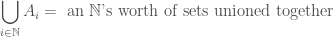
Of course, this process of union-ing over a finitely-indexed collection of sets works similarly for any sized index set, and, indeed, even for index sets that are not finite. Suppose we have a large collection of sets, one for each element in the counting or natural numbers $\mathbb{N}$ . We can then use our index, $i \in \mathbb{N}$ to name each set as, say, $A_i$ , and then we can form the infinite union

$\displaystyle \bigcup_{i\in\mathbb{N}} A_i = \bigcup_{i=1}^{\infty} A_i = A_1 \cup A_2 \cup A_3 \cup \cdots = \{x : x \in A_i \text{ for at least one } i \in \mathbb{N}\}$

While certain flavors of philosophers and logicians may contest this process, we, as budding mathematicians, are perfectly comfortable with it. Union-ing together an infinite collection of sets results in a new set, one with elements that came from at least one of the indexed sets (it could have also come from multiple).

Again, it is important to note that the sets $A_i$ may have absolutely nothing to do with the index set $\mathcal{I} = \mathbb{N}$ . The $A_i$ ‘s may be sets of real numbers, sets of rationals, sets of matrices, sets of words, etc; the index set is simply keeping track of these sets, it is not (necessarily) telling us anything about the elements in each set. Let’s explore two examples, one where the sets $A_i$ have nothing to do with the index $i \in \mathbb{N}$ , and one where the sets $A_i$ are, in fact, described in terms of the parameter $i \in \mathbb{N}$ .

Example (4). Let’s use the sets $A_1 = \mathbb{R}, A_2 = \{ ! \}, A_3 = \emptyset, A_4 = \mathbb{R}, A_5 = \{ ! \}, A_6 = \emptyset$ and so on. That is, our infinite collection of sets repeats itself according to the indicated pattern. We then have

$\displaystyle \bigcup_{i\in\mathbb{N}} A_i =\mathbb{R} \cup \{!\} \cup \emptyset \cup \mathbb{R} \cup \{!\} \cup \emptyset \cup \mathbb{R} \cup \{!\} \cup \emptyset \cdots = \mathbb{R} \cup \{!\}$

In some ways this was a very silly example. After all, we didn’t have infinitely many distinct sets to union, we just unioned together the same three sets over and over again. Still, this example helps solidify our two main points, which are worth repeating here.

The index parameter $i$ is not (necessarily) needed to write out the final set.
The index set (in this case $\mathcal{I} = \mathbb{N}$ ) does not (necessarily) determine the elements of any of the sets $A_i$ .

Example (5). Let us create an infinite family of sets each of which is described using the index $i \in \mathcal{I} = \mathbb{N}$ . Similar to our homework problems, let’s use

$\displaystyle A_i = [0, 1/i] = \{x \in \mathbb{R} : 0 \leq x \leq 1/i\} \subseteq \mathbb{R}$ .

For example, here are a few of the (infinitely many) sets we’ll be union-ing together:

$A_1 = [0, 1] = \{x \in \mathbb{R} : 0 \leq x \leq 1\}, A_{20} = [0, 20] = \{x \in \mathbb{R} : 0 \leq x \leq 1/20\}$ , and $A_{10000} = \left[0, \frac{1}{10000}\right].$

In this example, the index $i \in \mathbb{N}$ still has the responsibility of keeping track of the individual sets being unioned, but it also serves another purpose: each set $A_i$ is not just labelled with an $i$ , but its elements are also described in terms of the value of $i$ .

The index here is a natural number, $i \in \mathbb{N}$ , that is being used to label our sets and to define or describe our sets. However, the fact that $i$ is a whole number does not change or impact the fact that the sets being unioned contain elements that are not just whole numbers.

It is not too difficult o convince yourself that the larger $i$ becomes, the smaller the interval of real numbers $A_i$ becomes. Indeed, one can see that for any value of our index, it follows that $A_{i+1} \subseteq A_i$ (perhaps the easiest way to see this is to draw some pictures of these intervals). It then follows that

$\displaystyle \bigcup_{i\in\mathbb{N}} A_i = [0, 1] \cup [0, 1/2] \cup [0, 1/3] \cup \cdots = [0, 1]$

A Super-Infinite Union?

We now come to what I think is an especially tricky example, at least upon first glance. Although we are blessed / cursed with finite minds, thinking of an infinite collection of sets indexed by the counting numbers is not altogether too terrible. In Examples (4) and (5) above, we could have used the words

$\displaystyle \bigcup_{i\in\mathbb{N}} A_i = \text{ an } \mathbb{N}\text{'s worth of sets unioned together}$

to describe the process by which we produced the new, big-unioned set. Another way to talk about it is to say that we performed a discretely infinite union; after all, the natural numbers can be thought of as a discrete (albeit infinite) set of points that go on forever.

What happens, though, when our index set is even more complicated? For instance, what happens when we have a collection of sets $A_i$ not only for each natural number but for each real number, $i \in \mathbb{R}$ ? In this instance we could say something like this:

$\displaystyle \bigcup_{i\in\mathbb{R}} A_i = \text{ an } \mathbb{R}\text{'s worth of sets unioned together} = \text{ a real line's worth of sets unioned together}.$

We could also describe it as a continuous union of infinitely many sets. The main issue we have with this union / indexing is that we cannot write out something like

$\displaystyle \bigcup_{i\in\mathbb{R}} A_i = A_1 \cup A_2 \cup A_3 \cdots$

since doing so excludes the real-number-indexed sets like $A_{1/2}$ and $A_{e}$ . In other words, because we cannot (yet? ever?) list out the real numbers like we can the naturals, we are not able to write this union as an infinite list of unions. This, of course, is troublesome, but depending on the sets $A_i$ being used, the difficulties can be avoided.

Example 6. If we use, for example, $A_i = \{1, \$, g\}$ for every value of $i$ — that is, we have a “constant set”, then it follows

$\displaystyle \bigcup_{i\in\mathbb{R}} A_i = \bigcup_{i\in\mathbb{R}} \{1, \$, g\} = \{1, \$, g\}$

As in our examples that use finitely many indices and/or a natural-number’s worth of indices, the final set can be written out explicitly (and also without use of the index $i$ ).

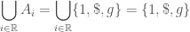
Example 7. Let’s consider a real line’s worth of one-element sets $A_i = \{i\}$ . For example, $A_0 = \{0\}, A_1 = \{1\}$ , and $A_{\sqrt{2}} = \{\sqrt{2}\}$ . Can you explain why

$\displaystyle \bigcup_{i\in\mathbb{R}} A_i = \mathbb{R} \text{ ?}$

Example 8. In this example we’ll use a real line’s worth of interval-subsets of the real numbers, specifically setting $A_i = [0, i^2]$ . Then

$\displaystyle \bigcup_{i\in\mathbb{R}} A_i = \bigcup_{i\in\mathbb{R}} [0,i^2] = [0, \infty)$ .

You should be able to convince yourself that this is true by thinking about the facts that (1) $A_i \subseteq A_{i+1}$ for every value of the index $i \geq 1$ , (2) $[0, i^2] \subseteq [0, (i+1)^2]$ for $i \geq 1$ . A picture of several of these intervals $A_i$ will likely help.

Example 9. We can, of course, also use not an entire real-line’s worth of sets, but, say, an intervals worth of sets. If we use $\mathcal{I} = [0, 1] = \{x \in \mathbb{R} : 0 \leq x \leq 1\}$ , then we can use any of the $A_i$ ‘s from the previous examples to form

$\displaystyle \bigcup_{i \in [0,1]} A_i$

For example, if we use the sets from Example 8 so that each $A_i = [0, i^2]$ is itself an interval of real numbers, you should be able to convince yourself that

$\displaystyle \bigcup_{i\in[0,1]} A_i = [0, 1]$ .

Second Day Musings

September 3, 2015 / d0mo / Leave a comment

Our second day of class went fairly well, I thought. Students appeared to be working well together, building consensus (or at least near-consensus) on the truth or falsity of four statements. As a refresher, here they are:

Given any triangle, there is always a circle that can be inscribed in it.
For ever integer $n \geq 2$ it is possible to choose $n$ points on a circle in such a way that if you connect every pair of points with straight line segments, the circle will be divided into $2^{n-1}$ regions.
Let $n \sharp$ be the product of the first $n$ primes. For every positive integer $n$ , $n \sharp+1$ is prime.
Every even number greater than 2 can be written as $p+q$ , where $p$ and $q$ are both prime numbers.

Since this class is all about proving things, I offer the following image as proof that, indeed, students were working on these true or false statements:

As we discussed in class, no one yet has an answer to the fourth statement. I don’t mean no one in our class, I mean no one, anywhere. (I suppose its possible that someone out there has an argument that demonstrates whether this is true or false and has chosen not to share it… let’s ignore that unlikely possibility.) Indeed, this is a famous conjecture, one called Goldbach’s Conjecture.

I think there is a good lesson here. Perhaps even multiple lessons. For instance, I think its important for FOM students to keep in mind that I might be trolling you. Yes, I had heard of this conjecture before compiling this assignment. Yes, I intentionally included it amongst other statements that can, actually, be argued true or false. Another lesson (hopefully?) learned here: mathematics is incomplete. There are lots and lots of mathematical statements that we can’t yet decide are true or false. In fact, this is what mathematical research is all about, finding new statements and proving whether or not they are true or false. What’s even better — and we’ll talk about this later in the semester — there are even mathematical statements that can never be proven true or false! Its crazy, I know, but there it is: sometimes a statement can never be proven true nor can it ever be proven false.

I will probably post another entry concerning my Blue Eyed Faculty story, but for now I raise my glass to this year’s FOM class(es). Cheers to an intoxicating semester!

More Great Math Quotes

January 28, 2013January 30, 2013 / d0mo / Leave a comment

These are taken from various FOM students.

“Math was here before we were here to describe it.” – Cyrus

“… the marks that dictate a mathematicians train of thought are far from meaningless … math is a necessary field of learning because it describes and proves why the physical world works the way it does.” – Kyle

“Math is trilling because it is capable of being shared with others, like my math buddy, and discussed to perfect clarity.” – Julia

“We don’t create these mathematical rules; we just discover them … Math follows basic simple rules and patterns and is thus consistent, yet certain ideas and concepts cannot be proved using these rules. It’s a mind-bending paradox – shouldn’t we be able to prove something if it is consistent?” – Cara

“This quote offers some powerful imagery. Mathematics is so beautiful because it allows us to impose order on the apparent chaos of our world. It is very comforting because – whether or not it is fatalistic – it shows us that there is in fact structure to the world around us. It can also be very humbling because of the complexity of it all, which can never be fully understood with an instrument as simple and imperfect as the human mind.” – Brad

“I have always viewed math as a challenge that can be overcome by working hard.” – Lauren

“Mathematics is already decided on, we’re just figuring it out.” – Leah

“Knowing something isn’t enough but you must also be able to prove it.” – Abiola

“My favorite math classes were not the ones where kids sat at their desk like a personal cubicle, but when people talked to each other and helped each other out about new concepts that were difficult and interesting.” – Ethan

“If x is an element of the null set, then this blog will be the best.” – Harry

“… when you can collaborate with others and learn from them, math is more inclusive and fun for everyone.” – Harry

“… with math there are millions of ways to explain one concept and sometimes hearing it a different way will finally help you understand. ” – Jennifer

“I really do believe that math is what is finally going to give us the true answers to the universe. Hell, according to some world-renowned works of literature the answer to life is the number 42.” – Nikolas

“Math has come to mean so much to me over my years of schooling. It is the root of science, economics and just LIFE. ” – Amanda

“Mathematics is not only a game, but a puzzle. Something to be cracked open and examined until the parts are fully understood. An element of excitement lies in the frustrating twists and turns traversed in the journey for Answers. Partly it is a personal, individual journey; it’s also a game played out across centuries, one thinker building on another and another and another to race for the right answer.” – Michelle

“Math, however, is not just a set of rules or principles to be memorized and then applied. In my classes when I solve new problems that I have never seen before I don’t just blindly apply a set of rules- I engage my own cognitive process to explore new concepts.” – Margaret

“While other subjects may ebb and flow with time, math is only refined with time.” – Matthew

“As the game of Mathematics is built on logic, just complying to basic rules will allow one to succeed at the game.” – Meteorologist Peekay

“David Hilbert, despite his brilliance, was sadly misinformed on the topic he knew best; an oxymoron of epic proportions.” – Zoe

“People all over the world, from beginners to mathematicians, work on problems non-stop as a game that is continuously being played…” – Ana

“In my opinion, there are no actually theorems or axioms in math. Math is just a set of numbers with some basic rules, which is designed or adjusted according to our observation to the nature. The theorems and axioms always exist even though we don’t know them. There is no one who produce the truths of math; they just discover them by their understanding and knowledge.” – Yingyi

Also, just a quick shout out: Kate’s blog is easily one of my favorites right now. I highly encourage you all to give it a look; not only does she have excellent lecture summaries and thoughts on the reading, but the images she includes are effing hilarious. Oh, and the same applies to the Mathasaurus Rex blog, too.

Runnin’ on Empty

September 16, 2012September 16, 2012 / d0mo / 2 Comments

Suppose $A$ is any set (it can be a set of familiar objects, like real numbers, it can be the empty set, or it can even be a set of something silly and/or pointless).

Is it true that $A \cup \emptyset = A$ ? If so, why? If not, why not? What does a proof for your answer look like?

Is it true that $A \cap \emptyset = A$ ? If so, why? If not, why not? What does a proof for your answer look like?

Lastly, a question I raised this past week: what is the set $A \times \emptyset$ ? Using our definition, we know that $A \times \emptyset = \left\{(x,y) : x \in A \text{ and } y \in \emptyset\right\}$ . Of course, this means that the element $y$ doesn’t exist, and so we might instead write $A \times \emptyset = \left\{(x, \,\,): x \in A\right\}$ .

This seems perfectly reasonable, and I, too, was tempted to draw this very same conclusion. However, it is wrong. Technically speaking, it violates the definition of Cartesian product. By specifying the second “entry” in the ordered pair $(x, \,\,)$ as “nothing” we are no longer talking about an ordered pair! An ordered pair is, by definition, a pair of things that exist. Hence, there are no ordered pairs in the set $A \times \emptyset$ , which means that $A \times \emptyset = \dots$ Ready for it? Have you figured it out yet?? That’s right! $A \times \emptyset = \emptyset$ !

Also, as many of you guessed, when you have two finite sets $A$ and $B$ (that is, two sets that each have finite cardinality), then the cardinality of their cross-product should be $\left|A \times B \right| = \left|A\right|\cdot\left|B\right|$ . Assuming this is true, and letting $B = \emptyset$ what do we learn about the cardinality of $A \times \emptyset$ ? In turn, what does this suggest must be true about the set $A \times \emptyset$ ?

So now I leave you with something to prove, and I’d like you to prove it a specific way. Given that proofs by contradiction are discussed in sections 2.3 and 2.4 of our textbook, this arrives at an ideal time.

Write a proof by contradiction that if $A$ is any set then $A \times \emptyset = \emptyset.$

This is not an officially assigned proof problem, but handing in a correct solution with your actual proof problems just might add some points to your grade. How many points? At the very least I promise to add $\left|A \times \emptyset\right|$ bonus points, if not more.

Guide to FOM Blogging

August 26, 2012September 1, 2015 / d0mo / 1 Comment

The single most important thing you will do in this course is keep a blog. Past FOM students almost universally agree that your blog/journal will be the hardest, most frustrating, and most vital part of this course. If you keep a thorough, up-to-date, organized blog it will serve as an incredible resource for you when you study for the midterm, while you’re completing the take-home final, and when you are taking later math courses. Here are some guidelines to help you make your blog as useful as possible.

Your blog should include various types of entries, which you may want to have clearly marked (possibly even color coded). Some suggested categories include the following:

Reading Notes. While you read the sections, you will take note of the important definitions and theorems. Copying these into your journal isn’t a waste of time – it will help you remember these things.

Reflections. The book periodically asks you to stop and reflect on some topic or question. When you do, take a moment to write down your thoughts.

Homework: I will frequently assign homework questions. These should be completed in your blog before you come to class; since typing mathematics can be time consuming (especially as you are learning to type it) you can discuss summaries of your problems and solutions in your blog posts. If you struggle on a problem, write what you can and leave space to fill it in later. During class we will typically take time to go over the homework, giving you a chance to fill in your gaps.

Classwork: We will frequently break up into groups in class to work on problems that I will put on the board. Your blog should include the work that you do in groups as well as notes from any class discussions we might have.

Be sure to title your blog entries so that they make sense to you, the TA, and myself. For instance, one post might look like this:

5 Sept.p. 51 I’m not sure if this is right, but I think that the truth set of

$\{x \in \mathbb{N} : |D(x)| \text{ is odd } \}$

includes all the odd perfect squares. This is because my hairdresser told me…

Your blog entires will be evaluated periodically (and somewhat randomly!) throughout the semester, so be sure to keep them current.

Frequency. You should have a well-written, thoughtful, and multifaceted entry for each class period (more or less). I hope “well-written” and “thoughtful” are clear, but if they are not, ask me for more information. By “multi-faceted” I mean your post should discuss more than one of the four “types” or “categories” described above. I understand and expect that some posts will be brief while others will be more fleshed out.

I also want to point out that the frequency requirements described above are a minimum. Longer, more frequent and complex posts are encouraged!

Tractor Beam

June 23, 2012 / d0mo / Leave a comment

Check it:

For more details on what this has to do with tractor beams and negative radiation pressure, consult Evelyn’s latest article.

Geodesic Loopiness: An Entirely Unnecessary Post

June 15, 2012June 16, 2012 / d0mo / Leave a comment

As I understand it, Mean Curvature Flow / Curve Shortening Flow was originally introduced as a means of producing and analyzing closed geodesics. Significant progress towards this goal was made throughout the decade 1980-1990 and owes much to the work of Gage, Grayson, Hamilton, Gluck, and Uhlenbeck (among others). Even better, their work inspired a number of new ideas and questions, (arguably laying the groundwork for the flows Perelman adjusted and used to solve the Poincare conjecture). To borrow a line from one of Dr. Gage’s talks, “the 80s were a good time for curvature flows.”

One such inspired question is this: Which curves exhibit self-similarity under this flow? The first person to tackle this problem appears to be the celebrated physicist William W. Mullins. He used mean curvature flow to model the motion of idealized grain boundaries in a 1956 paper, producing families of curves that either shrink of expand as they evolve.

Of course, the simplest example of a curve that shrinks under mean curvature flow is a circle. In 1986, Abresch and Langer classified all curves with this shrinking property, curves heretofore referred to as “shrinkers.” The vast majority of these shrinkers are stinkers, too, as they tend to be annulus-filling messes. Only a countable sub-collection behave nicely, like the ones pictured below.

Closed Shrinkers

The astute reader will note that these examples are rosette-like curves that live in various annuli, and the insanely astute reader might guess that the ratio $p/q$ that compares the number of petals to the curve’s turning number depends transcendentally on the maximum radial value and can only take values in the interval $\left[\frac{1}{2},\frac{1}{\sqrt{2}}\right].$ Indeed, such a reader would be correct.

Abresch and Langer’s methods involve differential/Riemannian geometry, as well as a few ad hoc techniques and computations relegated to appendices. A conjecture from their work stipulates that these shrinkers are certain kinds of saddle points, ones that lie “in between” circles and curves with cusps. This was affirmatively resolved in 2001 by Thomas Kwok-Keung Au, and curves featuring simultaneous types of similarity (shrinkers and expanders that also rotate) have recently been constructed by Halldorsson.

Most of the work in this area relies if not heavily on PDE theory then at least non-trivially, including the work of Au and Halldorsson. Interestingly enough, though, much of this dependency (and use of other “high level” mathematics) can be removed from Abresch and Langer’s original classification, so much of it, in fact, that their results become accessible to undergraduate math majors (relying upon elementary definitions from differential geometry or vector calculus, basic results in ODE theory, and calculus).

Au’s work contains the key to this simplification, a nifty geometric function called the support function. Given a hypersurface $X \subset \mathbb{R}^{n+1}$ the support function of $X$ is given by $h = \langle X, N \rangle$ where $N$ is a unit normal. For planar curves the support function is related to (signed) curvature via the equation

$k = -\frac{1}{h+h''}.$

Of course, mild restrictions apply. Most notably, the curve $X(u)$ must be locally convex so that it can be regularly parameterized by its unit normal $N(u) = e^{iu}$ . Assuming this and after applying a suitable rescaling, one discovers that $X(u)$ is a shrinker if and only if

$h'' = \frac{1}{h} - h.$

In fact, as noted in Au’s paper, for any locally convex curve evolving by Mean Curvature Flow, $h$ must satisfy the more general partial differential equation

$h_t = -\frac{1}{h+h_{u\,u}}$

where $h = h(u,t)$ with $u$ parameterizing the unit normal and $t$ representing time.

St. Mary’s math major Joshua Kaminsky and I spent the better part of the 2011/2012 academic year solving and studying the above ordinary differential equation (which can be obtained by seeking separable solutions to the above PDE). We were able to derive the Abresch-Langer classification, but we stumbled across quite a few new ideas and questions, too.

Before continuing, though, I should point out that I did not arrive at this problem honestly. That is to say that I was not thinking about mean curvature flow when this problem occurred to me. Rather, I came across it after attending various talks by Frank Morgan and his students. The equation $k+h = 0$ also shows up when seeking “weighted geodesics” (more specifically, but admittedly less clear, “Gaussian-weighted geodesics”). Indeed, the quantity $k+h$ is known as “weighted curvature.”

So-called Gaussian-weighted geodesics are curves that (locally) minimize

$\int \! e^{-r^2/2} \, ds$

This expression is nothing more than Euclidean arc-length that has been weighted by the Guassian (like) density $e^{-r^2/2}$ (it behooves me to mention that the $1/2$ factor is inconsequential; it corresponds to my choice of rescaling).

There is much more to share on this topic, and I intend to do so in upcoming posts, but I’m nearing a good stopping point now. A few notes before concluding, though.

First, Dr. Morgan’s REU students have made much progress on studying these (and other) “weighted” creatures, an area of study called “Manifolds with Density” (check out this paper and this one for starters). This casts our previous examples in a new light, making the unit circle and the more complicated but beautiful Abresch-Langer curves instances of Gaussian-weighted geodesics. In fact, Abresch and Langer’s original work proved an equivalent version of Dr. Morgan’s students’ conjecture (that was later proved) claiming that the circle is the only embedded Gaussian-weighted geodesic.

Second, Josh and I have a conjecture that constant weighted-curvature curves evolve through other constant weighted-curvature curves under the standard mean curvature flow, but they do so towards weighted geodesics. This aligns nicely with the previously mentioned conjecture made by Abresch and Langer and later verified by Au. We have also come across some interesting and strange findings in our attempts to classify all constant weighted-curvature curves. For instance, the bounds on that geometric ratio $p/q$ do not appear to hold.

Third, a 2012 St. Mary’s Undergraduate Research Fellow by the name of David Rice is currently wrapping up his exploration of some planar curves that exhibit translational self-symmetry under weighted curvature flow. These are curves that evolve according to the equation

$X_t = (k+h)N.$

After that is said and done we plan to tinker around with some of the constant weighted-curvature curve problems alluded to above.

Fourth, I have not even touched upon the current and massive amount of work being done on shrinking surfaces. While much PDE theory informs these results, geometric-oriented progress is currently under way (perhaps most notably by Colding and Minicozzi).

So, again I repeat, there’s a lot more to say on this! I hope to sketch out some explanations and ideas in future posts, all culminating in a few submitted papers, perhaps even a talk or two. For now, though, I’d like to reflect on a strange or unexpected loop that (hopefully) ties much of this together.

Here goes.

The hunt for geodesics involves a journey through other (specifically weighted) geodesics, which sounds a bit too self-referential for my liking … at least at first glance. Its perfectly harmless, of course, and quite ingenious when taken all together.

Evolving a closed curve by mean curvature flow will decrease its length (hence the alternate name “curve shortening flow”), and so if the curve isn’t destroyed in the process, it becomes a closed geodesic.
The question then shifts to one every destined-to-die victim in a horror movie asks, “What could go wrong?” That is, exactly how can a curve be destroyed? Curves flowing in a surface develop singularities pretty much how planar curves do, and so the question can be answered by analyzing the destruction of planar curves. It can be shown that when a closed planar curve dies it does so very much how a circle dies. That is, in the final moments of the curve’s life, it looks very much like a shrinker. Hence, if we can understand shrinkers, we can (better) understand closed geodesics.
Of course, shrinkers are themselves geodesics (with respect to a conformally Euclidean metric whose scaling factor involves a Gaussian density), and so the whole process can be repeated again. One attempts to find weighted geodesics by looking for shrinkers under weighted mean curvature flow (the same one David Rice is studying).

Very loopy indeed.

Except that its not. Not in the way you might think, at least. You’d expect this process to continue ad infinitum, but it turns out that a shrinker with respect to weighted-curvature flow was actually a shrinker (or maybe an expander) with respect to standard curvature flow all along (albeit with a change of scaling factor).

Not convinced? Here is the simple computation. Assume $X(u)$ is a shrinker with respect to weighted curvature flow, i.e.

$c'(t)X(u) = \frac{\partial X(u,t)}{\partial t} = (k(u,t)+h(u,t))N(u)$

where $c(t)$ is a smooth function. Evaluating this expression at $t=0$ , dotting with $N(u)$ , and letting $c'(0) = C$ produces the equation

$Ch(u) = \langle CX(u), N(u)\rangle = k(u)+h(u)$

which can be simplified to $k + (1-c)h = 0$ . When $1-c > 0$ this corresponds to old shrinkers, and when $1-c < 0$ we have an old expander. In either event, the game is over. We’ve “looped” back to our starting point.

So, to summarize all this loopiness about geodesic loops yet one more time: shrinkers help us understand how curves die (under mean curvature flow), in turn shedding light on geodesics. Similarly, then, “meta-shrinkers” should help us understand how curves die (under weighted mean curvature flow), shedding light on weighted geodesics. But meta-shrinkers are old shrinkers (or expanders). Hence, they often explain themselves!

All of this goes to show you how entirely unnecessary this post was. After all, its about something completely self explanatory.

Casey Douglas

Armageddon serious about maff